Estimación de volatilidad constante por métodos clásicos y bayesianos en un mercado financiero: Una aplicación a las preferenciales de Bancolombia
Constant volatility estimation by classical and bayesian methods in a financial market: An application to Bancolombia’s preferential prices
Christian Cortés-García
Universidad Surcolombiana (Colombia)
https://orcid.org/0000-0002-8955-4530
Alvaro Cangrejo-Esquivel
Universidad Surcolombiana (Colombia)
https://orcid.org/0000-0002-9237-0935
RESUMEN
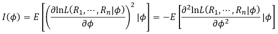
En este trabajo se proponen métodos, desde un enfoque clásico y bayesiano, para estimar la volatilidad constante de un activo cuando no es conveniente ajustar modelos de volatilidad heteroscedástica o estocástica en relación con la serie muestral del activo donde no se observa un aumento elevado de la volatilidad. Para probar cuál de los métodos propuestos se ajusta mejor a la variabilidad de la información y de los pronósticos, se utiliza el modelo estocástico propuesto por Paul Samuelson para estimar, con mínimo error, los precios de cierre de las acciones preferenciales de Bancolombia en un periodo muestral donde no se observa saltos significativos en la evolución de sus precios. Desde el enfoque bayesiano, se asumen a priori las distribuciones gamma inversa, estándar de Levy y de volatilidad de Jeffreys, con la estimación de los hiperparámetros propuestos por los autores. La metodología propuesta se contrasta con la estimación clásica de la volatilidad y el método bootstrap. A partir de los precios de cierre de la acción preferencial de Bancolombia durante un periodo de tiempo donde no existe significancia en el aumento o disminución en su volatilidad de manera temporal, la técnica bayesiana con distribución a priori Gamma Inversa captura la mayor información sobre la muestra de sus retornos, mientras que la estimación clásica de volatilidad pronostica el activo, dentro y fuera de muestra, con menor error. Sin embargo, los pronósticos del activo utilizando técnicas bayesianas o clásicas no muestran un impacto significativo.
PALABRAS CLAVE
Ecuación diferencial estocástica, lema de Ito, rendimientos, proceso estocástico, autocorrelación serial.
ABSTRACT
In this paper we propose methods, from a classical and Bayesian approach, to estimate the constant volatility of an asset when it is not appropriate to fit heteroscedastic or stochastic volatility models relative to the sample series of the asset where no large increase in volatility is observed. To test which of the proposed methods best adapts to the variability of information and forecasts, the stochastic model proposed by Paul Samuelson is used to estimate, with minimum error, the closing prices of Bancolombia’s preference shares in a sample period in which no significant jumps in the evolution of their prices are observed. From the Bayesian approach, the inverse gamma, standard Levy and Jeffreys volatility distributions are assumed a priori, with the estimation of the hyperparameters proposed by the authors. The proposed methodology is compared with classical volatility estimation and the bootstrap method. From the closing prices of Bancolombia’s preference shares over a period where there is no significant increase or decrease in volatility over time, the Bayesian technique with gamma inverse prior captures the most information about sample returns, while the classical volatility estimation forecasts the asset, in and out of sample, with less error. However, forecasting the asset using either Bayesian or classical techniques does not show a significant impact.
KEYWORDS
Stochastic differential equation, Ito’s lemma, returns, stochastic process, serial autocorrelation.
Clasificación JEL: C11, C12, C20, C51, G1.
MSC2010: 39A50, 91B30, 91B62, 91B84.
1. INTRODUCTION
The dynamics of the various economic factors affecting stock markets are of natural interest, given the role of these markets in stabilizing the financial sector to promote a country’s economic growth, whose behavior is uncertain and highly dependent on fluctuations in economic fundamentals (Bhowmik, 2013). In this context, the volatility of returns on financial assets is one of the most important uncertainty variables and therefore needs to be understood by market participants. Not only does it affect the efficient allocation of funds, but it can also hamper economic development as it plays a key role in the valuation of derivatives, the calculation of risk measures and the hedging of positions. In general, volatility is an estimate of the uncertainty of a financial asset and is quantified using statistical techniques. Chen (1997) and Chen, Du, Li & Ouyang (2013) stated that volatility should be calculated using the standard deviation of the series of returns in a financial series, since returns represent the fluctuations of the asset without scale and are much more manageable.
However, the assumption of constant volatility in traditional models such as Black & Scholes (1973) has been widely criticized in financial literature for its inability to capture phenomena observed in markets such as volatility smiles and smirks, volatility clustering and price jumps (Ho, Perraudin, & Sørensen, 1996; Eraker, Johannes, & Polson, 2003; Christoffersen, Heston, & Jacobs, 2013). Hull & White (1987) were pioneers in pointing out that volatility is not constant but varies over time and is subject to random shocks. This finding has led to the development of heteroskedastic and stochastic volatility models, where volatility is modelled as a random process with innovations independent of those of the return series (Awartani, & Corradi, 2005; Andritzky, Bannister, & Tamirisa, 2007; Álvarez Franco, Restrepo, & Pérez, 2007; Yang, Zhou, & Wang, 2009).
When the sample financial series exhibits significant and recurrent fluctuations over the period under study, the squared return series exhibits a significant serial autocorrelation structure, that is, a time dependence among its observations (Goudarzi, & Ramanarayanan, 2010; de Jesús Gutiérrez, 2015; Mamtha, & Srinivasan, 2016; Rossetti, Nagano, & Meirelles, 2017; Hendrych, & Cipra, 2018). In such cases, the volatility of the asset should be considered as time-dependent, and its estimation is carried out using heteroscedastic volatility models, such as those belonging to the GARCH family, or stochastic volatility models (Heston, & Nandi, 2000; Khan, Khan, & Khan, 2016; Garcia, & Esquivel, 2018a; ; ). Parameter estimation for these models is performed using maximum likelihood or Bayesian methods, considering distributions such as normal or generalized GED for the perturbations in this class of models (; ).
However, if there is no serial autocorrelation in the squared sample return series, that is, if the sample financial series does not exhibit significant or recurring fluctuations over the period under consideration, it is not statistically meaningful to fit stochastic or heteroscedastic volatility models (Goudarzi, & Ramanarayanan, 2010; de Jesús Gutiérrez, 2015; Mamtha, & Srinivasan, 2016; Khan, Khan, & Khan, 2016; Rossetti, Nagano, & Meirelles, 2017; Garcia, & Esquivel, 2018a; ; ; ). In such cases, volatility is assumed to be constant. However, even in this scenario, the estimation of constant volatility can be problematic, as the calculation of the standard deviation of returns can generate wide confidence intervals, making the precision of the sample estimate difficult. As the financial series in this study are not a function of intraday data or one-day high/low and opening and closing prices, HAR volatility models are not considered (; ).
To address this problem, some researchers have proposed alternative methods. For example, Karolyi (2019) uses prior information extracted from cross-sectional patterns of return volatility for groups of stocks sorted by size, financial leverage or trading volume, together with sample information, to derive the posterior variance density. This approach has shown higher predictive accuracy in option pricing than classical methods such as implied volatility or standard historical volatility. Similarly, Ho, Lee & Marsden (2011) use a Bayesian approach to estimate the constant volatility of stock prices by solving the heavy-tailed problem using the t-Student distribution. The authors show that volatility estimation using Bayesian methods is more accurate than classical methods.
In this context, our study proposes methods for estimating volatility when the sample return series follows a normal distribution and does not exhibit significant lags in squared returns. These estimates are made using classical and Bayesian methods, assuming as a priori distributions the inverse gamma, standard Lévy and Jeffrey distributions. These distributions are chosen to respect the fundamental properties of asset volatility, that is, non-negative and leptokurtic. In addition, the estimation method that best adapts to the variability of the information and predicts, with the minimum error, the daily closing prices of Bancolombia’s preferred shares between 02/01/2019 and 30/12/2019 (G. Bancolombia, 1875), which has no significant time jumps in its price evolution, is tested.
Our approach contributes to the literature by addressing the limitations of classical constant volatility estimation methods and by proposing Bayesian methods that improve the precision of the estimates. Moreover, the study is in line with recent literature highlighting the importance of independent volatility shocks and the flexibility of the correlation between returns and volatility (Eraker, Johannes & Polson, 2003; Christoffersen, Heston & Jacobs, 2013; Byun, Hyun, & Sung, 2021). By combining classical and Bayesian techniques, our work provides a flexible platform for estimating volatility in scenarios where heteroskedastic or stochastic models are not applicable in the sample time series.
2. RESEARCH METHODOLOGY
According to numerous studies (Goudarzi, & Ramanarayanan, 2010; de Jesús Gutiérrez, 2015; Mamtha, & Srinivasan, 2016; Khan, Khan, & Khan, 2016; Rossetti, Nagano, & Meirelles, 2017; Garcia, & Esquivel, 2018a; Garcia, & Esquivel, 2018b; Hendrych, & Cipra, 2018; García, & Esquivel, 2019; Byun, Hyun, & Sung, 2021), the following steps are suggested to determine whether volatility should be considered constant in a sample series of asset prices:
•Conversion of the sample time series of the asset into a series of returns (Tsay, 2014),
•Use the Dickey-Fuller test to determine that the series of returns follows a stationary process (Tsay, 2014),
•Use the Ljung-Box test to verify if the series of squared returns has significant lags in its autocorrelations (Tsay, 2014). If there are no significant lags, volatility is considered constant.
For the case where the return series follows a normal distribution with zero population means, this paper proposes alternatives using classical and Bayesian methods to estimate the constant volatility of an asset over a given period. If we are interested in estimating asset prices for a short period of time, the next section presents a difference equation for estimating returns, which is a discrete solution of a stochastic differential equation describing the asset returns and whose parameters are given by the sample mean and variance of the returns, together with a random behavior given by the interaction of volatility with fluctuations determined by a normal distribution.
3. MODEL DESCRIPTION
The following is a mathematical model that can be used to estimate the returns of an asset, the parameters of which are given by the sample mean and variance of the return series. Similarly, conditions are given to determine whether the population means, or variance should be considered constant.
3.1. Model for estimating sample returns
Consider a historical record of the monthly prices of an asset  , whose monthly asset returns
  are of the form
with monthly mean estimation
and monthly variance estimation
where the standard deviation σ is known as the volatility of the monthly return.
If returns  are standardized,
and the histogram of  coincides with the density function of a random variable ϵt∼N(0,1), then the monthly returns
  follow a normal distribution, with a monthly mean
  and a monthly variance
  . In this case
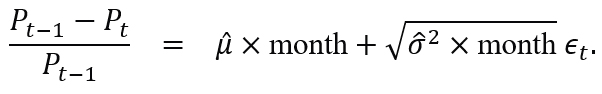
If Δt expresses a month and generally denotes the unit of time separating observations P0,P1⋯,Pn, by (3.3) we have that:
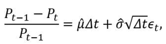
equivalently,
where ΔWt∼N(0,Δt), with E [ΔWt ]=0, and Var [ΔWt]=Δt.
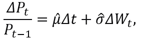
If Δt becomes smaller and smaller, for example, from months to weeks, from weeks to days, from days to hours, from hours to seconds, from seconds to moments, then the model (3.4) is equivalent to:
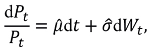
where d Wt∼N(0,dt) are the daily fluctuations in returns. The stochastic model (3.5) was introduced by Paul Samuelson (Venegas-Martínez, 2008).
In practice, we assume that μ and σ are known and that the only uncertainty in the model (3.5) is the random noise dW(t). Therefore, the simulation of the model (3.5) can be used to evaluate the stock price.
Using Ito’s Lemma (Venegas-Martínez, 2008), the model (3.5) is equivalent:
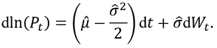
If dln(Pt)=ln(Pt)-ln(Pt-1) and S, then the discrete version of the model (3.6) is
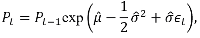
where ϵt∼N(0,1), and P0 is the initial price of the asset.
To predict asset prices using the model (3.7), we need to see that the parameters  and
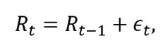
and  do not depend on time or position, that is, they are considered as constants. Therefore, we must check whether the series
  behaves as a stationary process and does not show significant autocorrelations between two periods t and s of the series Rt and Rt 2, respectively (Tsay, 2014).
According to Tsay (2014), to determine whether a series  is stationary, we must be checked that
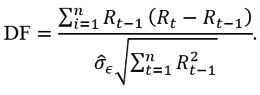
with ϵt∼N(0,1). For this purpose, the following model is considered
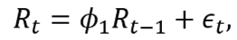
and the Dickey-Fuller test is proposed, which contrasts
with test statistician
To construct an estimator of ϕ1, note that the model (3.8) is equivalent to model
where Xt-1=Rt-Rt-1 and δ=ϕ1-1 is estimated by a simple linear regression without intercept.
An estimator of δ by the least squares method is
with R0=0, and
were
Since
then an estimator of  is given by
and
3.2. Constant mean and constant volatility conditions
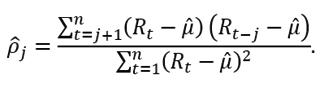
If is stationary, then the central idea behind fitting an ARMA model to account for μ as a non-constant parameter in is to test whether there are significant autocorrelations between two variables Rt and Rt-k, separated by k periods, defined by
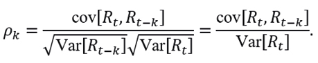
For this purpose, the Ljung-Box test is used, which tests the following hypothesis statement:
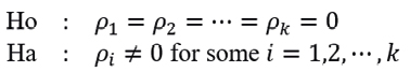
where k is the number of lags to test, with statistic
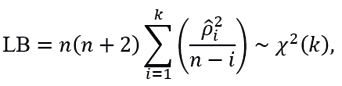
and
If has significant autocorrelations, then  is not considered a constant. Therefore, the mean of is fitted by an ARMA model such that
In addition, if there are significant autocorrelations in the series  , that is,
  , then is fitted by an GARCH family model, so
  is not considered a constant.
However, if follows a stationary process and has no significant lags, then  can be estimated by equation (3.2). In addition, if there is not enough evidence to reject the hypothesis for the series of returns, which contrasts
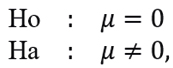
then we could consider μ=0.
Similarly, if the series  has no significant lags by means of the Ljung-Box test (3.11), then
  is considered as constant. Therefore, we must choose the best estimator of σ.
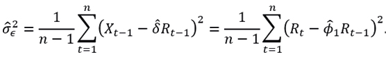
4. CONSTANT VOLATILITY ESTIMATION
We will show two techniques for estimating the constant volatility of an asset from the series of returns explained in Section 3.
4.1. Classical approach
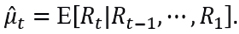
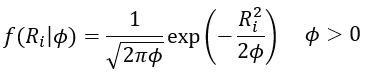
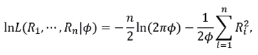
To perform the classical estimation procedure, it is necessary to define the probability distribution associated with the behavior of the returns Rt (3.1). If Rt∼N(0,ϕ), with ϕ=σ2,, then the density function is given by
To obtain an estimate of ϕ, the maximum likelihood method and the bootstrap technique are used as tools. The first method is to find  such that it maximises the likelihood function
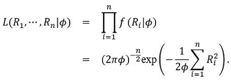
Indeed, since the equation (4.1) is equivalent to,
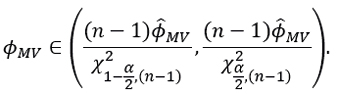
then
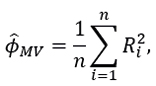
with confidence interval at 100(1-α)% given by:
On the other hand, if we consider bootstrap samples 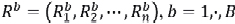 , as random re-sampling of (R1,R2,⋯,Rn), then by using an estimator
  , for example
  , to each bootstrap sample Rb, that is,
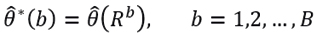
an estimator is proposed for ϕ given by
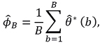
with quasi-variance
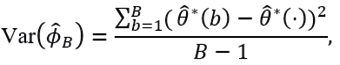
and confidence interval at a 100(1-α)% for ϕB given by
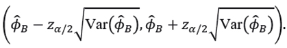
In particular, the above method is known as the bootstrap method (Efron, 1992).
4.2. Bayesian approach
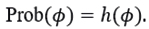
From the Bayesian approach (Bernardo, & Smith, 2009; Box, & Tiao, 2011), the parameter ϕ=σ2 is considered as a random variable modelled by a continuous prior probability distribution h(ϕ), whose information can be updated by observations from a sample (R1,⋯,Rn ). Consequently, we obtain a posterior distribution h(ϕ|R1,⋯Rn ) from which we have a complete description of the knowledge about ϕ obtained from the a priori distribution h(ϕ) and the sampling information (R1,⋯,Rn ).
From Bayes’ theorem we have that,
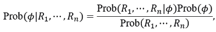
with
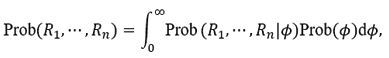
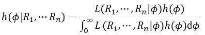
and
From the likelihood function L(R1,⋯,Rn |ϕ) (4.1), the population means of returns μ=0 and a prior distribution h(ϕ), the posterior distribution of ϕ can be found as follows:
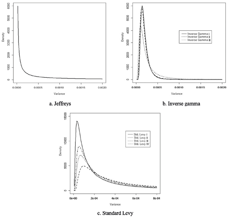
The following candidate prior distributions for the volatility of an asset are proposed by the authors below:
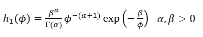
•Since ϕ>0, the a priori inverse Gamma distribution is a candidate for ϕ since it allows for skewness within its structure. The density function of the inverse Gamma distribution, for the variable ϕ is
From (4.1), the posterior distribution is
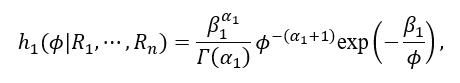
with  and
and  This distribution coincides with the Inverse Gamma distribution (4.3), with parameters (α1,β1 ).
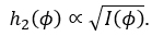
•One of the main strengths of Jeffreys’ method is its invariance under injective transformations, which is based on Fisher’s information measure on ϕ>0, that is,
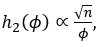
Thus, the prior distribution proposed by Jeffreys for the uniparametric case,
From (4.1), (4.4) and (4.5) we have that the a priori distribution is defined as
4.6
and from (4.2) we have
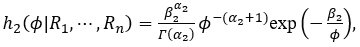
with  and
and  .
.
It is observed that the posterior distribution (4.7) is equivalent to the Inverse Gamma distribution (4.3) with parameters (α2,β2 ).
•Given that financial series can exhibit high volatility conditions, the a priori standard Levy distribution Levy(0,τ) is considered as a candidate because it exhibits heavy tails. The density function of the Levy distribution is defined as follows
with posterior distribution
which is an Inverse Gamma probability distribution (4.3), with  and
and 
5. PRESENTATION OF THE INFORMATION
The temporal series to be used are the daily returns of the preferred shares of the banking entity Bancolombia (G. Bancolombia, 1875). For the calculation of this return’s series (3.1), the daily closing prices of shares in which there is market in the period between 02/Jan/2019 and 30/December/2019 have been used, with a total of 245 observations (Bolsa de valores de Colombia, 2001).
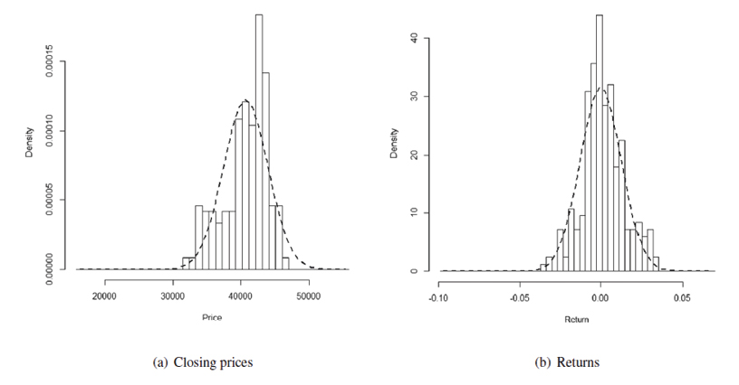
The histogram in Bolsa de valores de Colombia, 2001 shows that the price series data does not follow a normal distribution, but is slightly skewed to the left and leptokurtic, with a skewness coefficient of -0.6363245 and a kurtosis of 2.26349.
Figure 1. Price and return series PFBCOLOM
When modelling time series, it is important to determine whether the phenomenon under analysis follows a stationary process, that is, with unchanging meaning and variance in the period under study 0≤t≤244. To this end, using the Dickey-Fuller test (3.9), it is concluded that, at a significant level of 5%, the price series does not statistically behave with a time-varying mean and variance. In this case, Pt does not behave statistically as a stationary process with a probability of 25.63%. It is therefore of great interest to analyse the returns of the series using the returns of this stock.
Figure 2 shows the differences between the closing price series  and the return series
  , which statistically behaves like a stationary process with a probability <1% given by the Dickey-Fuller test (3.9) at a significance level of 5%.
Figure 2. Price and return series PFBCOLOM
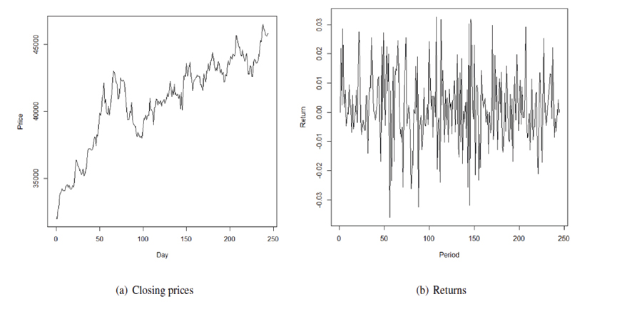
Table 1 shows that the series Rt behaves like a normal distribution, as it is slightly skewed to the left and platykurtic, with a skewness coefficient of 0.076 and a kurtosis of 0.347. However, the Shapiro-Wilk and Jarque-Bera test is used to determine whether the series Rt behaves like a normal distribution.
Table 1. Description of PFBCOLOM shares
|
Measure |
Statistician |
|
|---|---|---|
|
Closing Price |
Returns |
|
|
Media |
38767.78 |
0.001678714 |
|
Median |
39700 |
0.0005376344 |
|
Variance |
7774182 |
0.0001655227 |
|
Standard deviation |
2788.222 |
0.01286556 |
|
IQR |
4215 |
0.01316559 |
|
Skewness |
-0.6363245 |
-0.07809873 |
|
Kurtosis |
2.26349 |
3.361937 |
The probabilities associated with the Shapiro-Wilk and Jarque-Bera tests are 1.4% and 4.43%, respectively, which is insufficient evidence to determine that the series Rt does not follow a normal distribution, with a significance level of 5%.
Figure 3, the simple autocorrelation function (3.10) of the series Rt and  have few significant lags that are outside the 95% confidence intervals, however, the Ljung-Box test (3.11) is applied to check the significance of the autocorrelations up to lag 30.
Figure 3. Correlation of return and squared return series
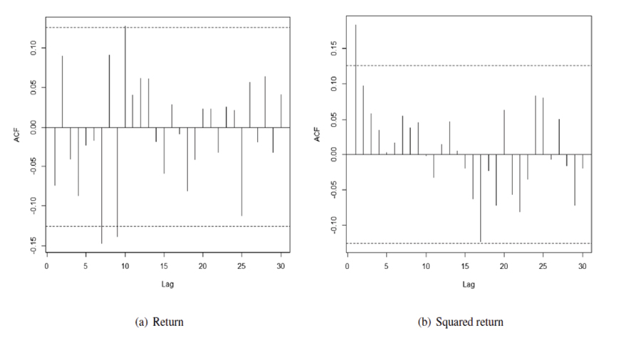
The probabilities associated with the LB test statistic for the series Rt and  are 65.41% and 40.89% respectively, which is insufficient evidence to determine that the series Rt and have significant lags at the 5% significance level, and therefore there is no presence of serial autocorrelation in either series. This suggests that an ARMA model for the mean and GARCH family models for the volatility of the returns should not be fitted. Therefore, μ and σ of the series Rt are considered as constants.
Applying a test tn-1 on the return series (3.12), it appears that, at a significant level of 5%, the population mean of Rt can be considered statistically zero with a probability of 5.6%. Next, we proceed to estimate the hyperparameters for each prior distribution to be considered to calculate the parameter σ.
6. HYPERPARAMETER ESTIMATION
Since the hyperparameters α and β of the inverse gamma prior (4.3) and τ of the Levy distribution (4.8) are unknown and no expert judgement is available to determine their values, the following methods are proposed to compute them (Tovar Cuevas, 2015).
We take the daily prices of Bancolombia’s preferred shares, obtained from the Bolsa de valores de Colombia (2001), during the period from 22/February/2010 to 28/December/2018, with a total of 2161 observations. From the data corresponding to the returns  , 72 excluded subsets of 30 elements each are formed, and, for each subset, the sample variance is calculated to obtain a vector of estimates
 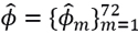 .
.
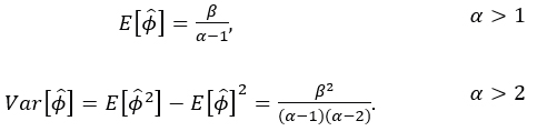
Based on the above, the first and second moments of the inverse gamma distribution (4.3) are calculated, that is,
6.1
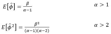
and determined the sample variance of the vector of estimates  as a function of moments, to form a system of linear equations with two unknowns given by:
The solutions of the system (6.2) are given by
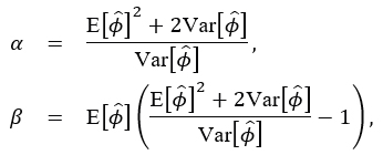
which defines a first case for the hyperparameters of the Inverse Gamma prior distribution (4.3).
A second case consists in calculating the historical volatility for each 20 days of the above series of returns, that is,
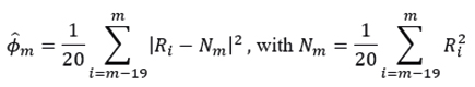
to obtain a vector of estimates  . and estimate α and β as posed in system (6.2).
A third case consists in taking a sample of the returns corresponding to the period 02/January/2018 and 28/December/2018, that is,  and the mean and variance are calculated to replace them in the system (6.2) to obtain a third Inverse Gamma prior distribution (4.3).
To obtain prior information about the parameter τ of the Standard Levy distribution (4.8), we divide the set , generated in the first case, into 8 exhaustive excluding subsets with 9 elements each, that is,  , i=1,⋯,8 and, for each of the sets, we estimate
  by the maximum likelihood method, that is,
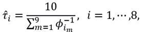
and the minimum, maximum, mean, and median values of these estimates are taken to establish values of the hyperparameters of the Standard Levy prior distribution.
Table 2 shows the estimates for the hyperparameters of the Inverse Gamma (4.3) and standard Levy prior distributions (4.8). In the first case of the Inverse Gamma distribution, the parameter α is the largest compared to the other Inverse Gamma prior distributions, which causes the distribution to be more leptokurtic, that is, it has a smaller variance in its structure compared to the others as observed in Figure 4(b). In the Standard Levy distribution, as the hyperparameter  becomes smaller, the distribution tends to become leptokurtic, as observed in Figure 4(c).
Table 2 Estimates of hyperparameters for each prior distribution
|
Distribution h(ϕ) |
Hyperparameter |
|---|---|
|
Inverse Gamma I |
(α,β)=(5.255163,0.000859) |
|
Inverse Gamma II |
(α,β)=(4.481333,0.000704) |
|
Inverse Gamma III |
(α,β)=(2.000404,0.000306) |
|
Standard Levy I |
τ=0.000103 |
|
Standard Levy II |
τ=0.000295 |
|
Standard Levy III |
τ=0.000203 |
|
Standard Levy VI |
τ=0.000163 |
7. RESULTS
Using the mean as a measure that summarizes the σ2 information for each of the posterior distributions, Table 3 shows the estimates of the volatilities by the proposed methods, where the estimation was done by the bootstrap method with B=200 and the initial estimator generated by the maximum likelihood method  .
.
Table 3 shows that the are quite similar for the different methods. However, the 95% confidence regions for the Bayesian models tend to have less variability than those observed by the 95% confidence intervals given by the classical methods, which allows a better precision in the volatility estimation.
Table 3. Estimation of σ ̂2 from the different methods proposed
|
Method |
Type |
σ ̂2 |
Interval estimator |
|---|---|---|---|
|
Classic |
Maximum Likelihood |
0.000158796 |
(0.0001339515,0.0001912957) |
|
Bootstrap |
0001586208 |
(0.0001260133,0.0001912284) |
|
|
Bayesian |
Jeffreys |
0.0001618451 |
(0.0001515057,0.0001934298) |
|
Inverse Gamma I |
0.000161998 |
(0.0001518425,0.0001929266) |
|
|
Inverse Gamma II |
0.0001616447 |
(0.0001515535,0.0001924145) |
|
|
Inverse Gamma III |
0.0001617566 |
(0.0001515217,0.0001932139) |
|
|
Standard Levy I |
0.0001602782 |
(0.0001501442,0.0001913579) |
|
|
Standard Levy II |
0.0001610221 |
(0.0001507602,0.0001920557) |
|
|
Standard Levy III |
0.0001607126 |
(0.0001505169,0.0001918419) |
|
|
Standard Levy VI |
0.0001605483 |
(0.0001503757,0.0001914762) |
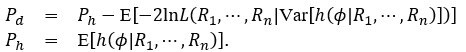
Since each of the priori distributions has the same posteriori distribution, with different hyperparameters, it is necessary to determine which a posteriori distribution is the most appropriate for the estimation of the volatility parameter. From a Bayesian point of view, the Deviance information criterion (DIC) is used, which is based on the posterior distribution, since the log-likelihood of the model is a measure of model fit to the data, and the deviance is a measure of discrepancy between the model and the data.
The DIC criterion is calculated using the expression
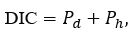
Where
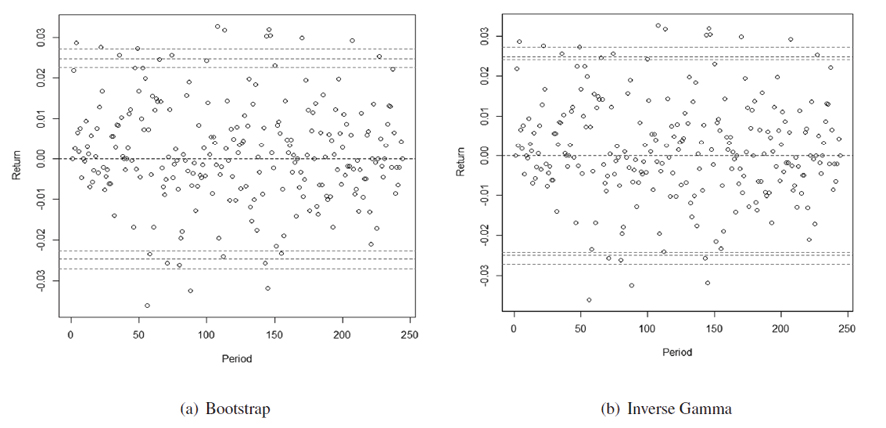
Since that the bootstrap method has lower variability in the confidence interval than the maximum likelihood method, and the Inverse Gamma III prior distribution has a lower DIC, as observed in Table 4, Figure 5 shows the confidence bands for the volatility of the returns, at a 95% confidence level of both the point estimates and the extremes of the confidence bands for both methods. The two selected estimation methods do not capture the totality of returns. However, when analyzing the extremes of the intervals of the σ estimates, the Bayesian method can capture more information than the classical method. Therefore, the Bayesian method, in addition to showing less variability in its 95% confidence intervals, manages to capture more information about returns than the classical method.
|
Previa |
Posterior |
DIC |
|---|---|---|
|
Jeffreys |
Inverse Gamma |
12532.52 |
|
Inverse Gamma I |
Inverse Gamma |
12519.46 |
|
Inverse Gamma II |
12564.64 |
|
|
Inverse Gamma III |
12517.85 |
|
|
Standard Levy I |
Inverse Gamma |
12765.72 |
|
Standard Levy I |
12651.82 |
|
|
Standard Levy II |
12723.19 |
|
|
Standard Levy III |
12724.53 |
Figure 5. 95% confidence bands for return volatility
On the other hand, if the initial asset price is  , corresponding to 28/December/2018, the model (3.7) with
  is used to estimate the closing prices and compare its results with the real prices within the sample, that is, from 02/January/2019 to 30/December/2019, where
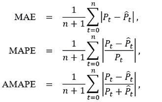
are the errors of these forecasts, with actual closing prices Pt and forecast closing prices  .
.
Considering 1000 numerical solutions, with fixed random values ϵt∼N(0,1) for each solution, we can be seen from Table 5 that the σ estimator using the bootstrap technique has the lowest means of MAE, MAPE and AMAPE, with respect to the Maximum Likelihood method and the Bayesian methods, which have lower DIC in each of their prior distributions, confirming that this method predicts Bancolombia’s stock prices with minimum error.
Table 5. In-sample forecast errors by classical and Bayesian methods
|
Method |
Type |
MAE |
MAPE |
AMAPE |
|---|---|---|---|---|
|
Classic |
Maximum Likelihood |
5159.698 |
0.1247814 |
0.06561538 |
|
Bootstrap |
5157.789 |
0.1247363 |
0.06559164 |
|
|
Bayesian |
Jeffreys |
5192.784 |
0.1255642 |
0.06602711 |
|
Inverse Gamma III |
5191.827 |
0.1255416 |
0.0660152 |
|
|
Standard Levy II |
5183.877 |
0.1253535 |
0.06591627 |
However, if we compare the residuals 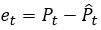 for each of the 1000 asset price predictions made by each Bayesian volatility estimation method with lower DIC and the bootstrap method relative to the actual prices between the period 02/January/2019 to 30/December/2019, then from the mean of the 1000 Diebold-Mariano (DM) tests (Diebold, & Mariano, 1995; Harvey, Leybourne, & Newbold, 1997), we conclude that the two forecasts have the same accuracy as observed in Table 6.
Table 6. Comparison between the accuracy of in-sample asset price forecasting using the bootstrap method and Bayesian estimation
|
Distribution h(ϕ) |
Mean p-valor Diebold-Mariano test |
|---|---|
|
Jeffreys |
0.3943 |
|
Inverse Gamma III |
0.3875 |
|
Standard Levy II |
0.3842 |
By performing 5000 numerical solutions of the model (3.7), for  as estimated by the bootstrap method, and by computing the computational mean and variance for each partition t∈[0,243], Figure 6(a) shows the relationship between Bancolombia’s actual closing prices, during the period 02/January/2019 to 30/December/2019, and one of the predictions along with the 95% confidence interval. Although an adequate fit was not achieved, due to noise generated by model (3.7), such estimates can be considered by investors for decision making.
Figure 6. Forecasts closing price by Bootstrap method
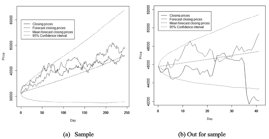
Finally, considering as initial asset price P0=45800, corresponding to 30/December/2019, we contrast the classical and Bayesian volatility estimation methods to estimate the closing prices by model (3.7) and compare their results with prices between 02/January/2020 to 28/February/2020, for a total of 41 data.
When considering 1000 numerical solutions, with fixed random values ϵt∼N(0,1) for each solution, and as shown in Table 7, it is evident that the bootstrap method, besides forecasting with lowest means error the in-sample asset prices, also forecasts the out-of-sample asset prices with lowest means of MAE, MAPE and AMAPE errors. However, as shown in Table 8, the mean Diebold-Mariano (DM) test, which compares the 1000 forecasts of each Bayesian method with respect to the bootstrap method, confirms that both classical and Bayesian estimation methods predict out-of-sample asset prices similarly. Figure 6(b) compares the actual asset prices to those predicted by the out-of-sample bootstrap method, which 95% confidence interval captures much of the information from the actual prices.
Table 7. Out-of-sample forecast errors by classical and Bayesian methods
|
Method |
Type |
MAE |
MAPE |
AMAPE |
|---|---|---|---|---|
|
Classic |
Maximum Likelihood |
2811.727 |
0.05746561 |
0.03001113 |
|
Bootstrap |
2810.969 |
0.05745062 |
0.03000334 |
|
|
Bayesian |
Jeffreys |
2824.885 |
0.05772597 |
0.03014635 |
|
Inverse Gamma I |
2825.543 |
0.057739 |
0.03015312 |
|
|
Inverse Gamma II |
2824.022 |
0.0577089 |
0.03013749 |
|
|
Inverse Gamma III |
2824.504 |
0.05771843 |
0.03014244 |
|
|
Standard Levy I |
2818.133 |
0.05759236 |
0.03007696 |
|
|
Standard Levy II |
2821.341 |
0.05765584 |
0.03010993 |
|
|
Standard Levy III |
2820.007 |
0.05762944 |
0.03009622 |
|
|
Standard Levy IV |
2819.298 |
0.05761542 |
0.03008894 |
Table 8. Comparison between the accuracy of out-of-sample asset price forecasting using the bootstrap method and Bayesian estimation
|
Distribution h(ϕ) |
Mean p-valor Diebold-Mariano test |
|---|---|
|
Jeffreys |
0.2972 |
|
Inverse Gamma I |
0.2822 |
|
Inverse Gamma II |
0.2964 |
|
Inverse Gamma III |
0.2737 |
|
Standard Levy I |
0.2844 |
|
Standard Levy II |
0.2785 |
|
Standard Levy III |
0.2972 |
|
Standard Levy IV |
0.2923 |
8. CONCLUSIONS
Since there is not much research on the estimation of constant volatility, apart from the classical method and through resampling methods, it is interesting to propose alternatives to be contrasted with the classical estimates. One of these alternatives is to propose estimates using Bayesian methods, since from a priori distribution of the possible behavior of the volatility, a posteriori distribution is determined, which is generated by the information of the sample returns, and which can be used to estimate the volatility.
For each posteriori distribution, the Bayes estimator was evaluated with respect to the quadratic loss function, that is, the expected value of the distribution is taken as a measure that summarizes the volatility information (Tovar, 2015), although other possible statistics to estimate the volatility could be accepted. At the sensitivity level, such methods, both classical and Bayesian, could be contrasted by the smaller range of their confidence intervals or regions, as there would be less variability in the sample estimate of volatility.
Confidence intervals for the classical approach (CI) and credible regions by estimating the IQR of the posterior distribution are used in the Bayesian approach (CR) to assess the quality of volatility estimates, although CI and CR are concepts with completely different interpretations. The CI sets two values for the estimator within which it is expected to find the random quantity of interest a certain percentage of the time, whereas the CR should generate a proportion of values of the unknown quantity equal to a specified probability. Although conceptual confidence intervals and credible regions are different, for practical reasons their lengths and the average coverage obtained after many iterations of the estimation procedure can be used as indicators of the performance of the estimates obtained.
On the other hand, the choice of the priori distribution for volatility is made based on experience or on the suggestion of the researcher or an expert. In this case, given that the Jefrey, Gamma - Inverse and Standard Levy distributions have been chosen as prior distributions to describe volatility, other possible distributions similar in nature to those chosen in this work could be proposed as future work, that is, they should not contain negative values in their structure. In addition, due to the lack of information from an expert, an empirical Bayesian method (Tovar-Cuevas, 2015) was proposed for the selection of the hyperparameters of the priori distributions.
In the case of constant volatility to describe the risk of an asset, the normal distribution has been considered as a candidate to describe the returns and thus construct the likelihood function to calculate the a posteriori distribution. However, other possible distributions could be considered as the series generally behave as leptokurtic or with heavy tails. As possible future work, the Laplace or GED generalized distribution could be considered to describe the return series.
Therefore, since the Colombian Stock Exchange only presents price records on business days, equation (3.1) is used to estimate simple returns. On the other hand, if asset prices are recorded daily, the logarithm of simple returns could be considered as an estimator of returns, since the origin of this formula is related to the continuous interest rate, which is used in many financial fields as the interest rate that operates different instruments, in this case stock returns, although from a mathematical point of view both estimates are equivalent.
From an economic point of view, the difference between constant volatility and time volatility applied to the return series is that the series does not show any significant variability, i.e. the increase in the price of the asset does not show any drastic fluctuations because external economic factors have not caused a significant increase or decrease in the price of the asset, as in the case of the price series of Bancolombia during the period implemented, so that there are no significant autocorrelations in the series of returns squared of the preference shares of Bancolombia, it does not make sense to fit a volatility model, so it should be considered as constant and either classical or Bayesian estimation techniques should be applied.
In the comparison of Bayesian methods for estimating the volatility of the series of returns on Bancolombia’s preferred shares, when the inverse gamma prior distribution is taken, it presents a lower value in the DIC, indicating that the distribution has a better fit than the others. However, the classical method was able to make predictions with minimal error compared to the Bayesian methods. On the other hand, regardless of the hyperparameters in the different procedures, it has been demonstrated that the results do not present significant differences and that the proposed methodology can be applied in different fields of study where the variable of interest presents positive asymmetric behavior.
REFERENCES
, , & (2007). Estudio de efectos asimétricos y día de la semana en el índice de volatilidad’VIX’. Revista Ingenierías Universidad de Medellín, 6(11), 126-147.
, , & (2007). The impact of macroeconomic announcements on emerging market bonds. Emerging Markets Review, 8(1), 20-37.
, & (2005). Predicting the volatility of the S&P-500 stock index via GARCH models: the role of asymmetries. International Journal of forecasting, 21(1), 167-183.
, & (2009). Bayesian theory (Vol. 405). John Wiley & Sons.
(2013). Stock market volatility: An evaluation. International Journal of Scientific and Research Publications, 3(10), 1-17.
, & (1973).The Pricing of Options and Corporate Liabilities. Journal of Political Economy, 81(3), 637-654.
Bolsa de valores de Colombia, https://www.bvc.com.co/pps/tibco/portalbvc, [Online; accessed 2-August-2019] (2001).
, & (2011). Bayesian inference in statistical analysis. John Wiley & Sons.
, , & (2021). Estimation of stochastic volatility and option prices. Journal of Futures Markets, 41(3), 349-360.
(1997). Empirical Performance of Alternative Option Pricing Models. Journal of Finance, 52(5), 2003-2049.
, , , & (2013). Does foreign institutional ownership increase return volatility? Evidence from China. Journal of Banking & Finance, 37(2), 660-669.
, , & (2013). Capturing Option Anomalies with a Variance-Dependent Pricing Kernel. Review of Financial Studies, 26(8), 1963-2006.
, & (2021). A practical guide to harnessing the HAR volatility model. Journal of Banking & Finance, 133, 106285.
(2015). Predicción de la Volatilidad de los Precios del Petróleo Mexicano: CGARCH Asimétrico con Distribuciones Normal y Laplace. Ciencias Administrativas. Teoría y Praxis, 11(1), 93-112.
, & , (1995). Comparing Predictive Accuracy. Journal of Business and Economic Statistics, 13, 253-265.
(1992). Bootstrap methods: another look at the jackknife. In Breakthroughs in statistics: Methodology and distribution (pp. 569-593). New York, NY: Springer New York.
, , & (2003). The Impact of Jumps in Volatility and Returns. Journal of Finance, 58(3), 1269-1300.
, & (2017). Ajuste de modelos GARCH Clásico y Bayesiano con innovaciones t-Student para el índice COLCAP. Revista De Economía Del Caribe, (19), 1-32.
, https://www.grupobancolombia.com/wps/portal/personas, [Online; accessed 28-June-2019] (1875).
, & (2018a). Propuesta de un modelo de volatilidad a los precios de cierre en las acciones CÉMEX LATAM HOLDINGS durante el periodo 15/noviembre/2012 al 27/octubre/2017. Ingeniería y Región, 19, 22-34.
, & (2018b). Modelo de volatilidad en un mercado financiero colombiano. Comunicaciones en Estadística, 11(2), 191-218.
, & (2019). Modelo de volatilidad a los precios de cierre de la acción pfcemargos comprendidas entre 16/mayo/2013 al 31/mayo/2017. Cuadernos de Economía, 42(119), 119-138.
, & (2010). Modeling and estimation of volatility in the Indian stock market. International Journal of Business and Management, 5(2), 85-98.
, & (1997). Testing the equality of prediction mean squared errors. International Journal of Forecasting, 13(2), 281-291.
, & (2018). Self-weighted recursive estimation of GARCH models. Communications in Statistics-Simulation and Computation, 47(2), 315-328.
, & (2000). A Closed-Form GARCH Option Valuation Model. Review of Financial Studies, 13(3), 585-625.
, , & (1996). A Continuous-Time Arbitrage-Pricing Model with Stochastic Volatility and Jumps. Journal of Business & Economic Statistics, 14(1), 31-43.
, , & (2011). Use of Bayesian estimates to determine the volatility parameter input in the black-scholes and binomial option pricing models. Journal of Risk and Financial Management, 4(1), 74-96.
, & (1987). The Pricing of Options on Assets with Stochastic Volatilities. Journal of Finance, 42(2), 281-300.
(1993). A Bayesian approach to modeling stock return volatility for option valuation. Journal of Financial and Quantitative Analysis, 28(4), 579-594.
, , & (2016). Pricing of risk, various volatility dynamics and macroeconomic exposure of firm returns: New evidence on age effect. International Journal of Economics and Financial Issues, 6(2), 551-561.
, & (2016). Stock market volatility–conceptual perspective through literature survey. Mediterranean Journal of Social Sciences, 7(1), 208-212.
, , , & (2019). Versatile HAR model for realized volatility: A least square model averaging perspective. Journal of Management Science and Engineering, 4(1), 55-73.
, , & (2017). A behavioral analysis of the volatility of interbank interest rates in developed and emerging countries. Journal of Economics, Finance and Administrative Science, 22(42), 99-128.
(2015). Inferencia Bayesiana e Investigación en salud: un caso de aplicación en diagnóstico clínico. Revista Médica de Risaralda, 22 (1), 9-16.
(2014). An introduction to analysis of financial data with R. John Wiley & Sons.
(2008). Riesgos financieros y económicos, productos derivados y decisiones económicas bajo incertidumbre (Vol. 1). Escuela Superior de Economía, Instituto Politécnico Nacional.
, & (2006). Bayesian inference on mixture-of-experts for estimation of stochastic volatility. In Econometric Analysis of Financial and Economic Time Series (Vol. 20, pp. 277-296). Emerald Group Publishing Limited.
, , & (2009). The stock–bond correlation and macroeconomic conditions: One and a half centuries of evidence. Journal of Banking & Finance, 33(4), 670-680.